INTRO
Imagine you want to simulate a speaker, utilizing Thiele-Small parameters. It’s traditional and “easy” to obtain a frequency response graph with a lumped element model and a Laplace transform, but we live in the time domain, and you can’t hear a graph. I’ve stumbled into a method for directly translating any lumped element model of an LTI system into a set of filters which allow you to model the system’s response in time! Not only can we obtain the frequency response of a driver, but we can listen to it directly. Imagine being able to simulate a few speakers and select the one that sounds best!
In addition to an efficient means for auralization directly from the lumped-elements, I offer a unique solution to simulating the impedance of a loudspeaker.
THE LUMPED ELEMENTS
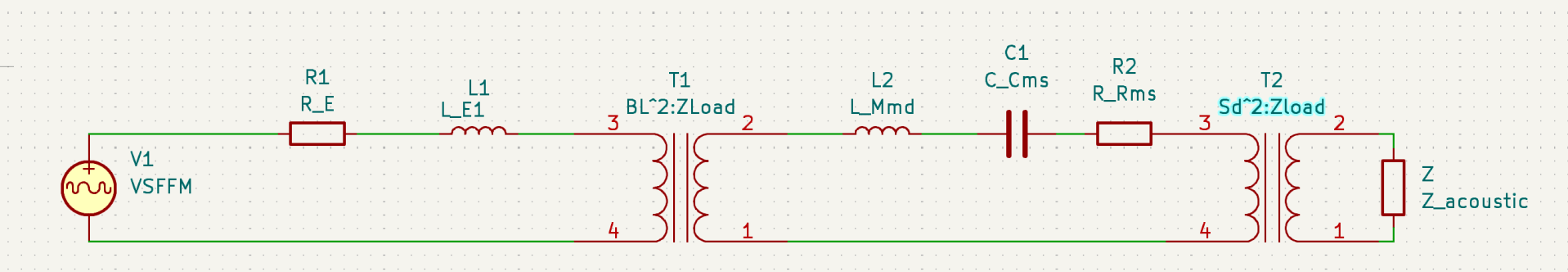
In the basic assumption of a lumped element model for a loudspeaker, where the 3 domains of a speaker are “analogized” to circuit elements, coupled via a gyrators (transformer shown due to Kicad limitations), the above circuit can be simulated (choose your poison) to examine transducer behavior in any of the three domains. The trick here is that the behavior of a speaker in the time domain is a mess of differential equations but circuit elements themselves have very nice solutions once you flip over to the frequency domain. Let’s start with a simple example.
A SIMPLE EXAMPLE AS A JUSTIFICATION FOR USING FREQUENCY DOMAIN
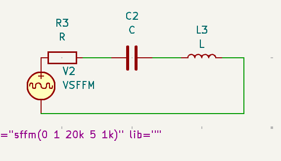
For example, for an RLC circuit (R=0Ω for simplicity, resistance is a constant with respect to frequency/time/etc)
The time domain analysis looks something like this, where I is current and V is voltage.
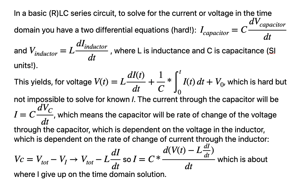
The main issue here is that to calculate current you must evaluate an expression which itself requires knowledge of the derivative of the current. This is a differential equation! It’s not impossible to compute this numerically (that is, assume a small δ and step through time little by little) but obtaining an “analytical” solution to the equation requires a special set of skills.
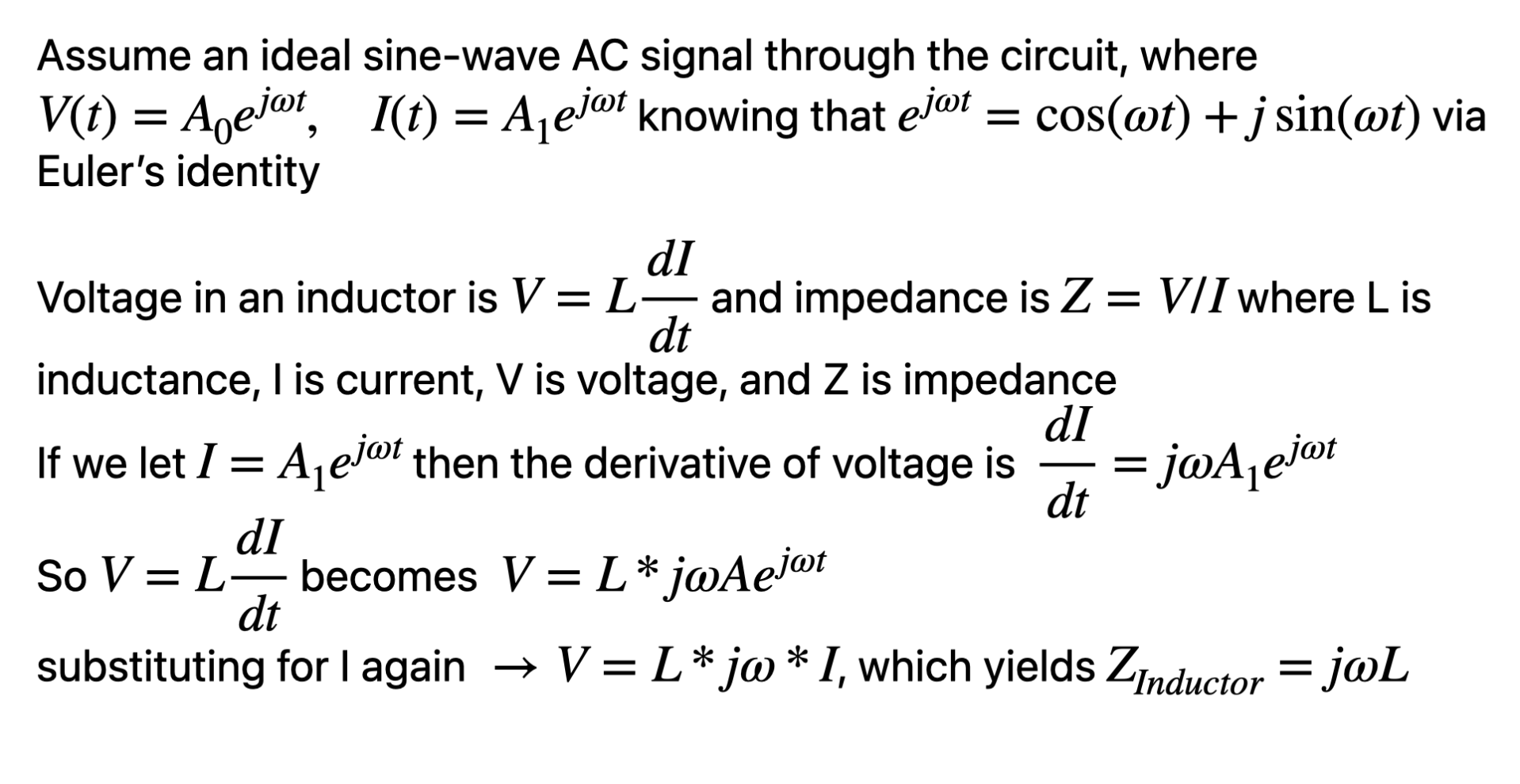
If instead you instead do some clever stuff with frequency, based on 1) Euler’s Identity and 2) the understanding from the Fourier Theorem that any signal may be represented by an infinite series of sine waves, there are some very handy and very useful solutions to differential equations. (warning: I’m using j notation for imaginary numbers)
Here’s my mini proof, where j is the square root of negative 1, ω is frequency, and t is time:
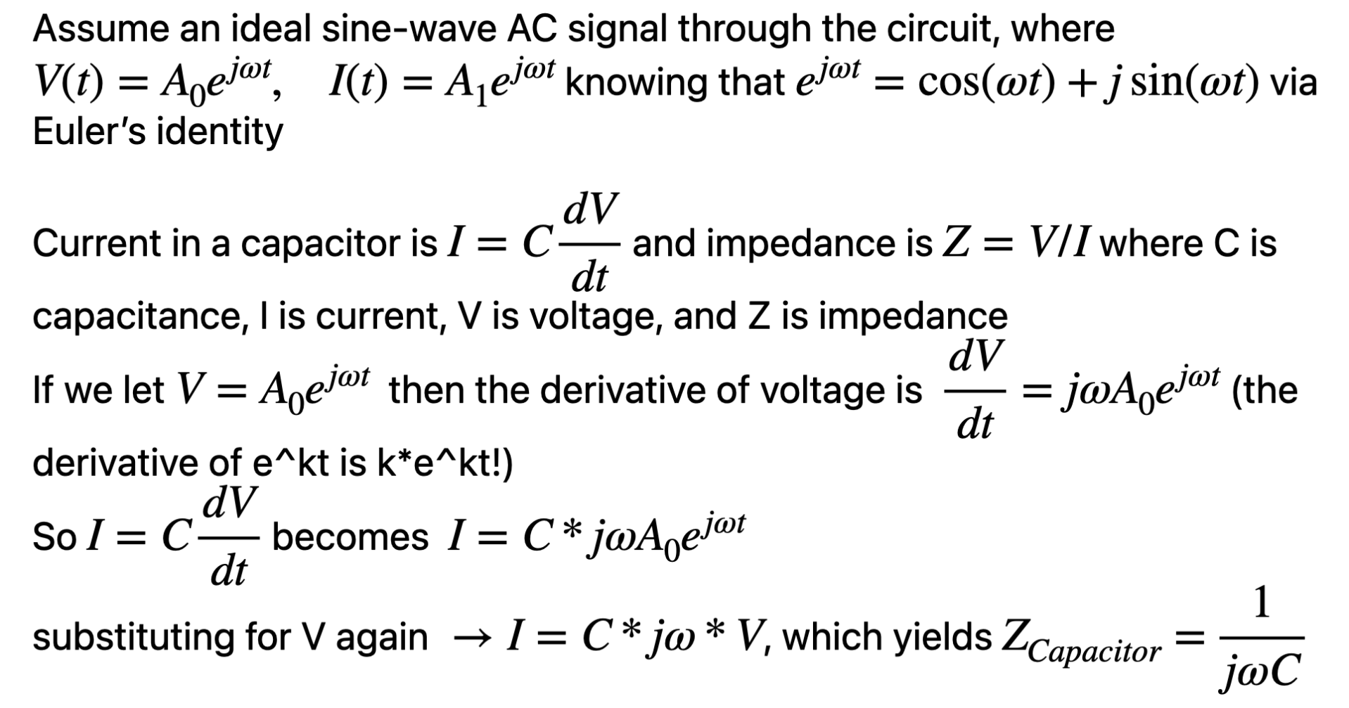
By taking advantage of the Euler identity and the very special property of e that its derivative is itself, we can evaluate the differential equations and reduce them to simple polynomial math (more on that later).
Since we now know the complex impedance of these circuit elements, the series circuit can be “solved” as such:

The final expression is a fully accurate solution to the circuit, and it tells us a lot about the behavior of the circuit. For instance: for a given current and frequency, increasing capacitance will lower voltage (the capacitor will proportionately charge less) and lowering frequency will increase voltage (capacitor will charge more!) but this is counteracted by the decreasing impeance of the inductor. Makes sense, but let’s visualize it to get the whole story!
If the poison you so choose is a frequency domain analysis, you can easily plot the frequency domain response by substituting s = j*2*pi*f where f is an vector of sample points in Herz (e.g. f=[1,2,3…48kHz]). Here’s some simple Matlab code to do this:
f = 1:fs; %sample points
omega = 2*pi.*f; %convert to angular frequency
s = 1i*omega;
C=100e-6; %Farads
L=10e-4; %Henries
R=1; %Ohms
Z=1./(s*C)+s*L+R; %series circuit impedance

An interesting note before we go to the Laplace domain: the impedance of this circuit looks a lot like a (logarithmic) graph of a quadratic function. In fact, if we replace jω with a variable…say s, it can be written as:

So, we’ve turned a differential equation into a polynomial equation!
BUT WHAT ABOUT TIME?
Bing, bang, boom! Frequency response of a lumped element circuit with an elegant polynomial solution! But what about time the time domain? And the filter I promised?? Armed with a frequency response (hitherto known as FR), it is certainly possible to create a time domain transfer function or filter. Here are some methods I’ve tried:
Methods to convert a Frequency Response (FR) to a time-domain filter
| method | big O | pros, cons |
| IFFT(FR) → time domain convolution with signal | O(m*n) m is resolution of FR n is signal samples | + simple, rather direct – accuracy limited by FR resolution – super slow – i hear you like ringing and group delay |
| DFT(signal) x FR | O(m log n) | + relatively easy to understand and implement – not “real-time” i.e. requires “frames” with overlap and add – time domain artifacts due to finite signals, finite resolution |
| FIR2: Frequency sampling-based FIR filter design | O(m log n)? | + brute force solution – memory intensive filtering: very high order filter required for any reasonable accuracy (N==Fs) – accuracy limited by FR resolution |
| filter coefficient optimization: run steepest descent optimization on filter coefficients until filter matches FR | ∞ for optimization (optimality not guaranteed) O(n)* once filter is converged∞ *technically O(m*n) but filter order can be kept as low as order of system | + kind of cool + extra brute force solution – optimizing the filter is not a guaranteed-to-work process depending on FR complexity |
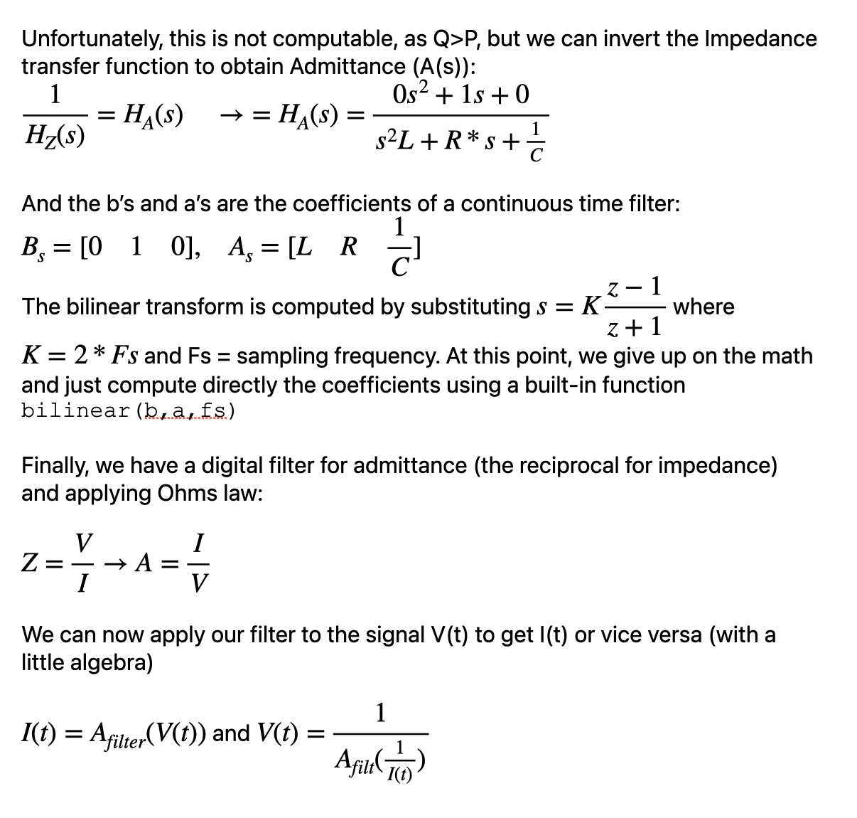
None of these are especially satisfying to me because they’re all rather messy approximations with a few levels of abstraction. This is the meat and potatoes of this post. There are two handy dandy pieces of math we need: the Laplace transform, which converts from time domain to the complex frequency s-domain, and the bilinear transform which converts directly from the LaPlace s-domain equation to the discrete time domain of digital signals (airhorn noises). This is huge! We already did the frequency domain math for Rs, Ls, and Cs!
There’s just one thing: the Laplace domain is in terms of the complex frequency variable 𝑠 where 𝑠=𝜎+𝑗𝜔. We are allowed to convert from the Fourier domain to the LaPlace domain if we set 𝜎=0, which is more-or-less an assertion that the system is stable and the input is continuous (in time) and real (in frequency). Then we can simply replace every 𝑗𝜔 with an 𝑠:

This last expression is what is sometimes referred to as the polynomial solution. Let’s take that into the time domain:
Example code:
C=100e-6; %Farads
L=10e-4; %Henries
R=1; %Ohms

%polynomial expression
a=[L R 1/C]  %denominator
b=[0 1 0]   %numerator

[B,A]=bilinear(b,a,fs);

%results — this is all you need to filter any signal!
B =   0.0103    0.0000   -0.0103
A =   1.0000   -1.9751    0.9794
Checking the results shows alignment (of course!)
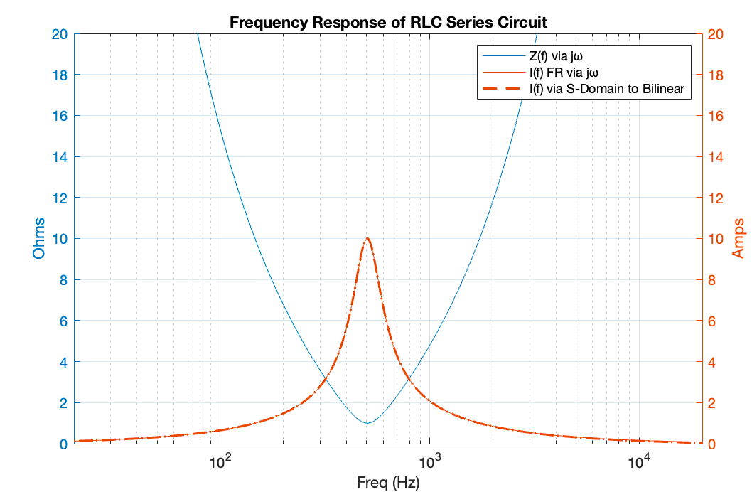
Ain’t that great? What I love about this method is that this is the exact analytical answer to “how will this circuit behave in response to a signal?” There are no cons I have discoverd (except for sampling frequency and subsequently the accuracy of the bilinear transform)!
| method | big O | pros, cons |
| Bilinear transform of polynomial solution | O(n)* technically m*n where m is the order of the system | + it’s the exact solution + super fast + gives you F(f) and F(t) + sounds cool – you have to “solve” the circuit |
To bring it home, we can also filter any time signal with our RLC circuit, giving us the time response. Here’s a 10V stepped input:

Or a stepped sine wave:
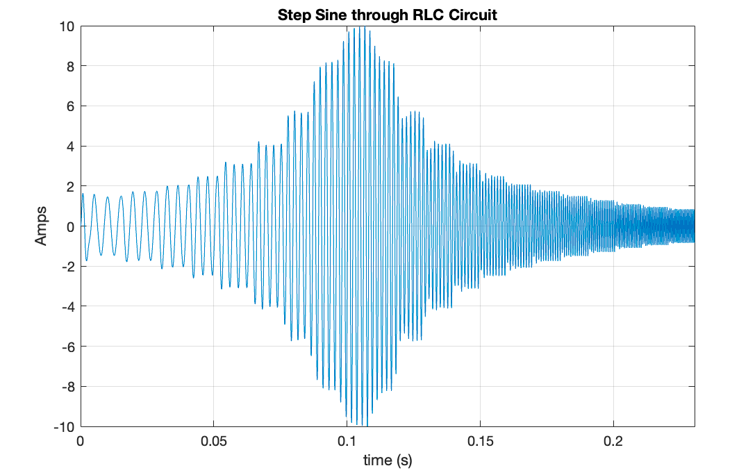
Admittedly, the bilinear transform is a discrete time approximation of a continuous time object—and so is a digital signal— but in comparison, say to a the FIR2 approach, which requires, for similar levels of accuracy, a 48,000-order filter fit to the response of the circuit, I find it much more satisfying to have a 6-term filter derived directly from the physical properties of the circuit.
APPLYING THIS METHOD TO ACOUSTICS
Now that we have a method that’s copacetic for a simple example, let’s apply this to the electro-mechano-acoustic domain! This is where the cons come in. While the math is simple and exact, the algebra quickly becomes nightmarish for complex systems. A simple transducer model is relatively simple until you chase down the acoustic terms, and then it becomes hellish, but I have a solution for that, too. Observe:


Factoring this chonky conglomeration to obtain coefficients yields something so grotesque it cannot be displayed readably with LaTex:

But using the power of the symbolic library, we can easily collect the terms and calculate the coefficients:

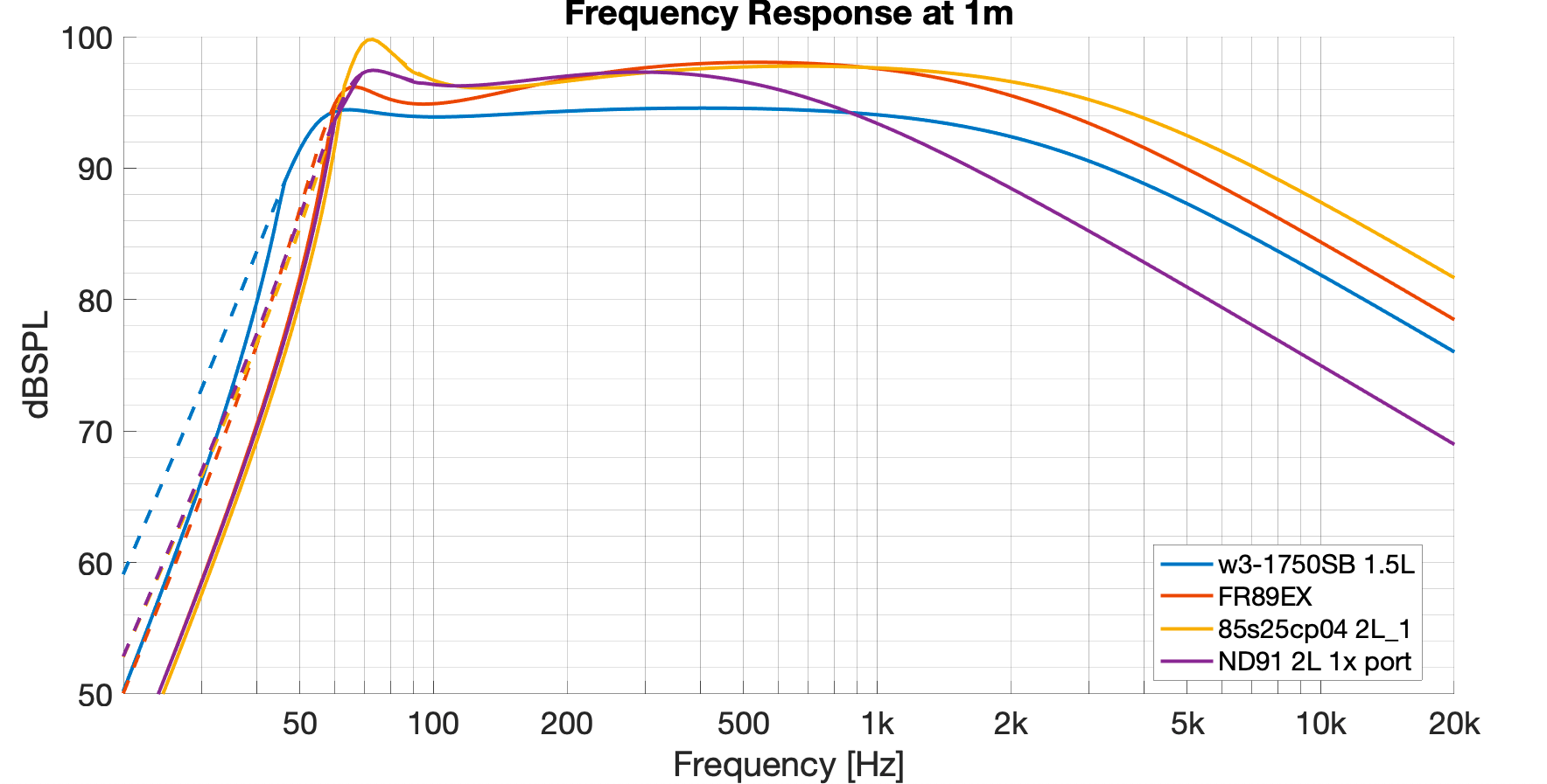
Turning Z(s) into a time domain filter Z(t) is as simple as taking the bilinear transform of 1/Z again! The results are validated with a comparison to a full speaker simulation software. If you’re wondering where the orange line is, it’s directly beneath the yellow line.
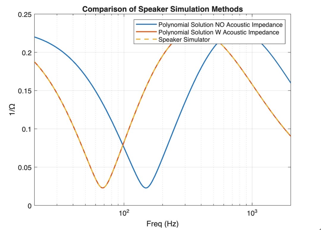
Admittedly, the model with acoustic impedance added is very close to the one without, but we’re here for precision anyway!
Inverting to impedance:
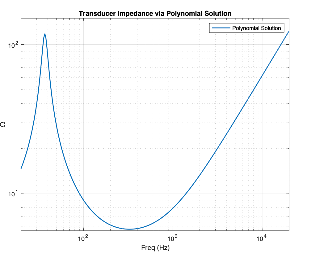
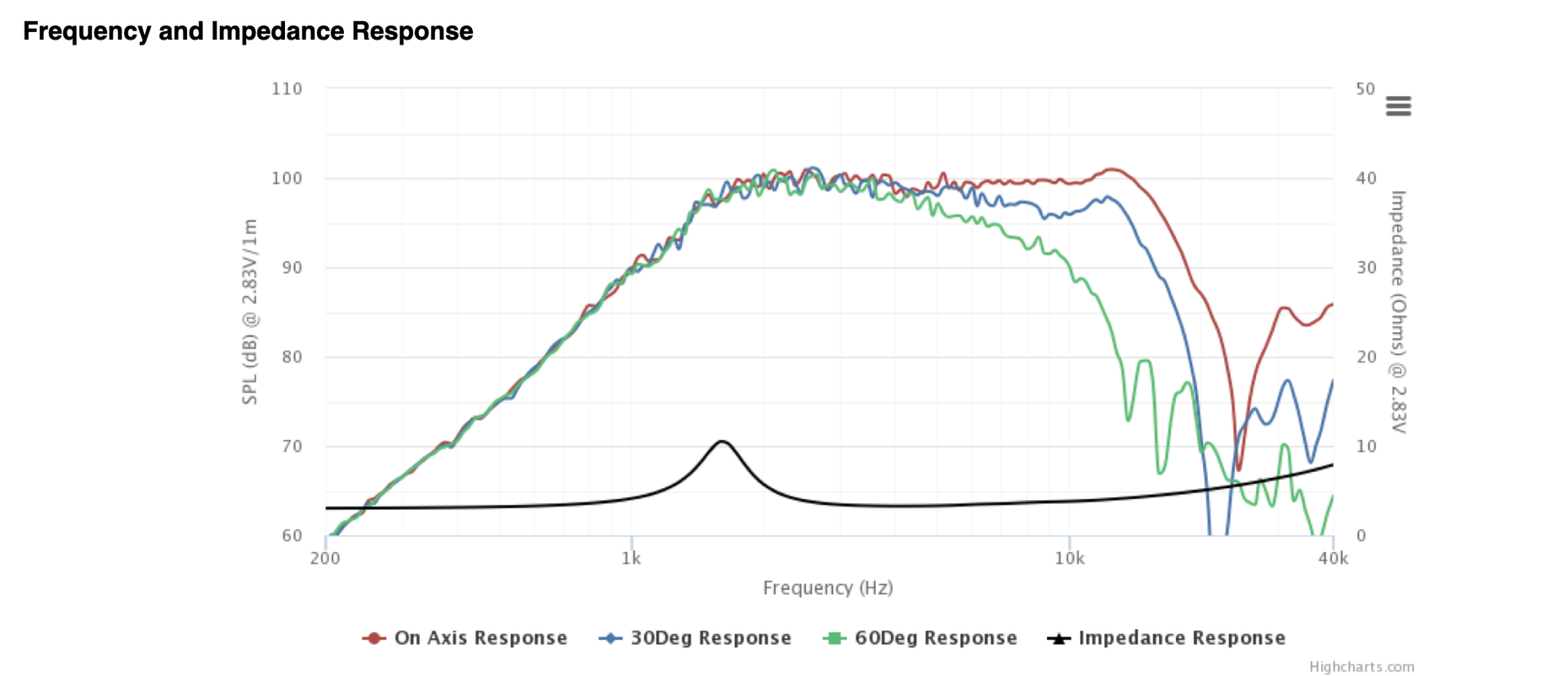
Checking it against a real transducer (I switched TS parameters for this one to the ND91-4 by Dayton Audio, a classic mini-woofer)—overlaying the simulated response on top of the DATS measured impedance response (blue line) by Dayton Audio vs our orange polynomial line, it looks pretty damn close up to 1kHz! The loss off accuracy above 1k is most likely due to the secondary inductance/resistance of the magnetic circuit, which is not typically reported by manufacturers in the TS parameters or datasheets and therefore not modeled.

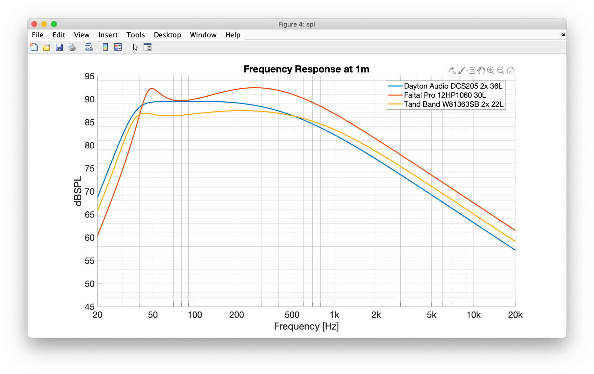
Et voila! with a little bit of computer assisted algebra, we can take a lumped element model and convert it into a time-domain filter to be applied directly to incoming signals. In this case, we solved the algebra to get us the time-domain impedance of a transducer model, but with some simple re-arranging and a little code we can convert voltage to excursion, SPL, velocity, transmitted force, and much more!


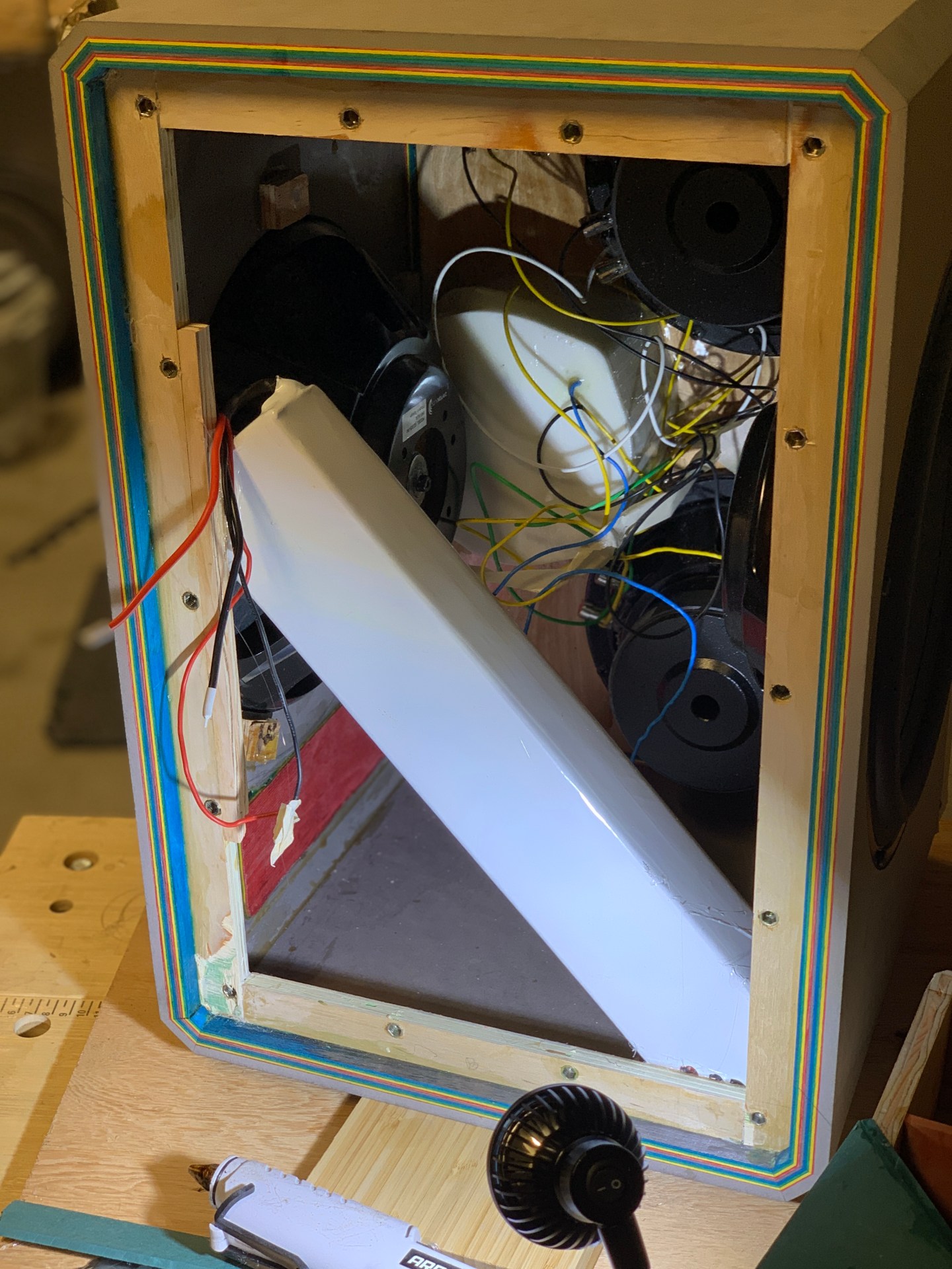


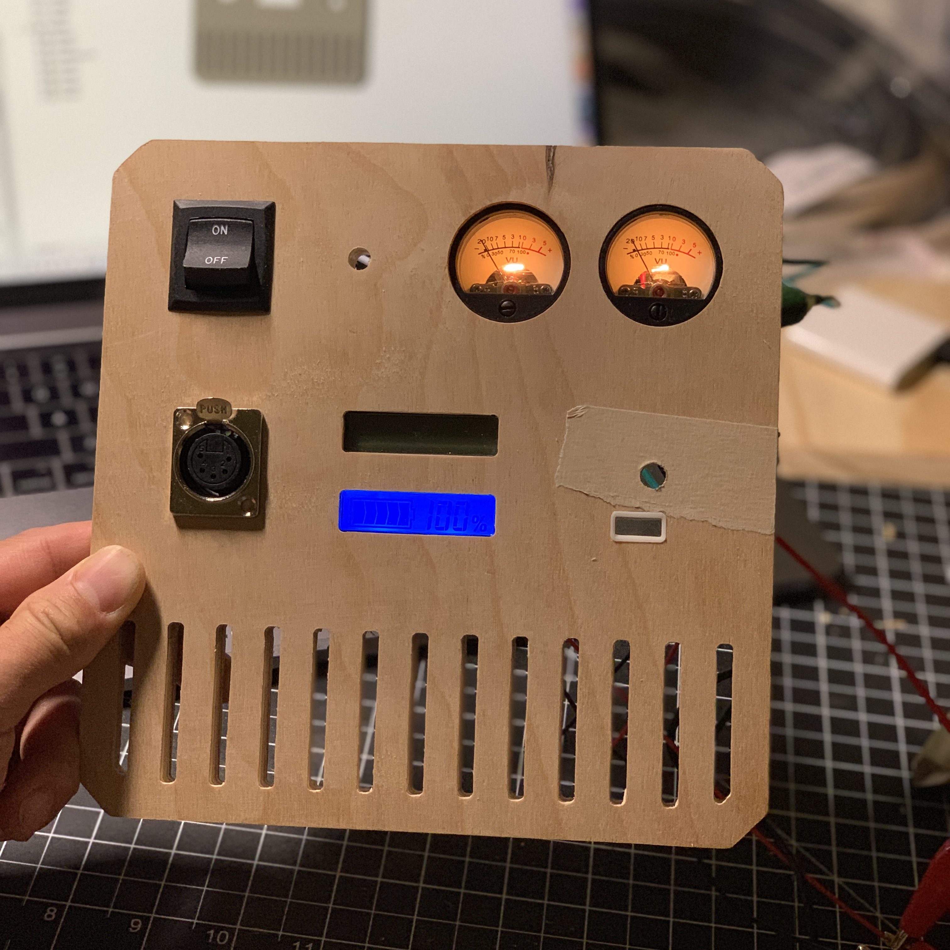


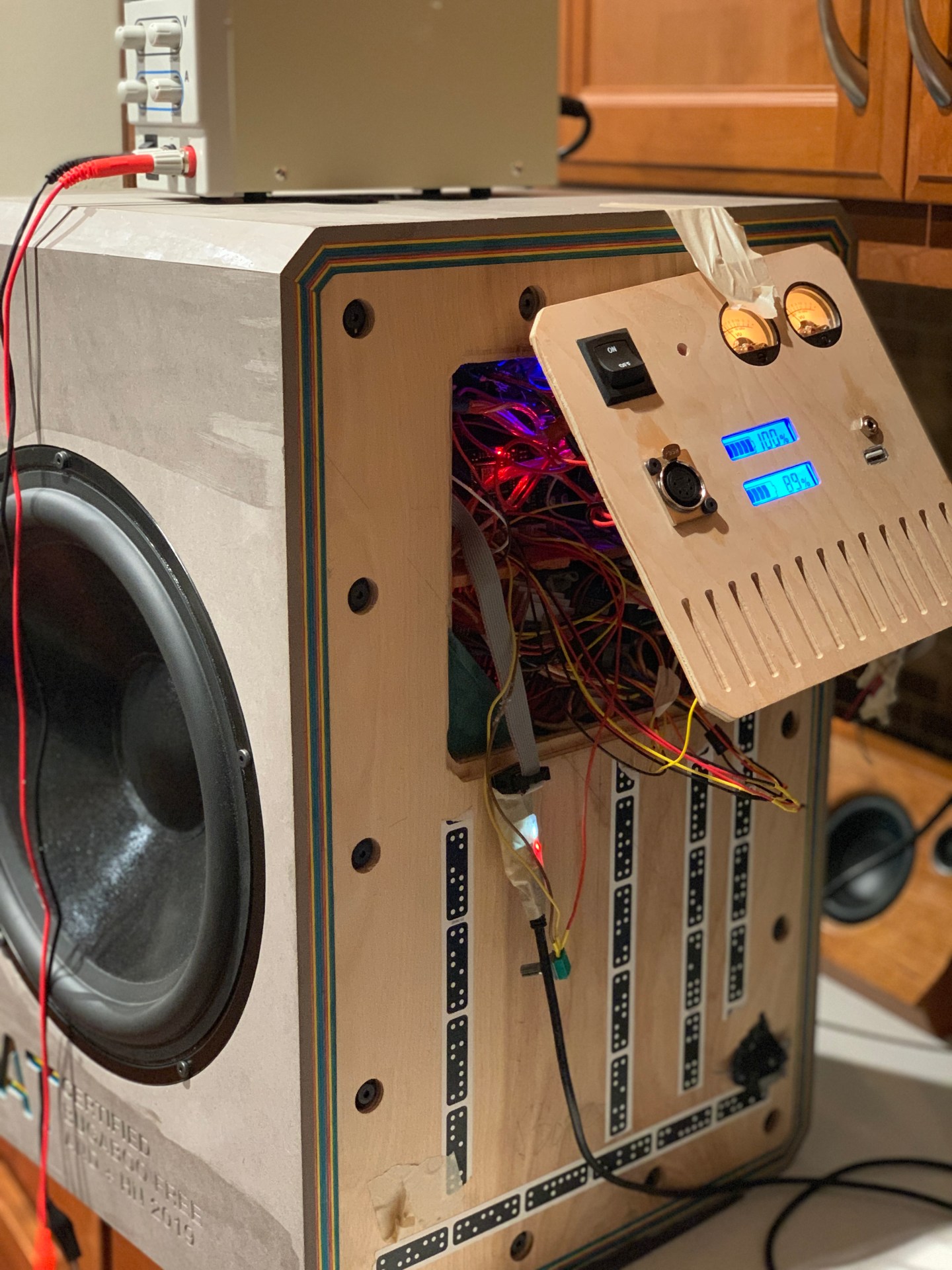
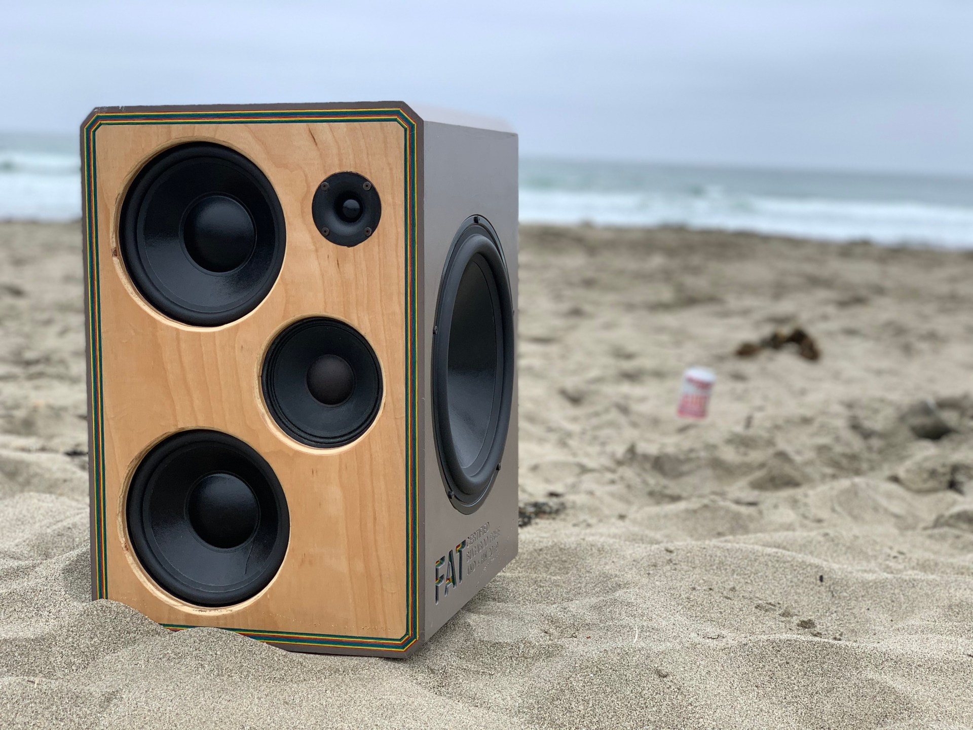


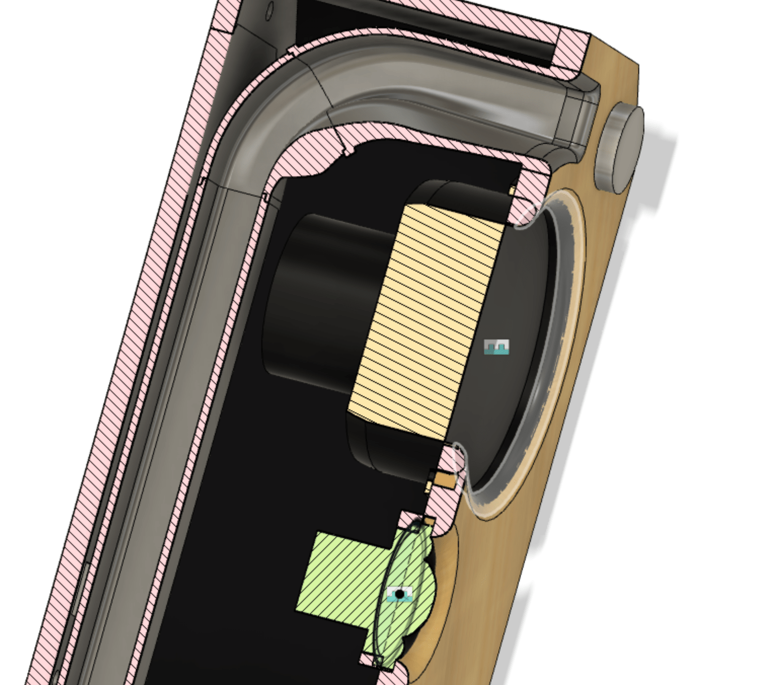
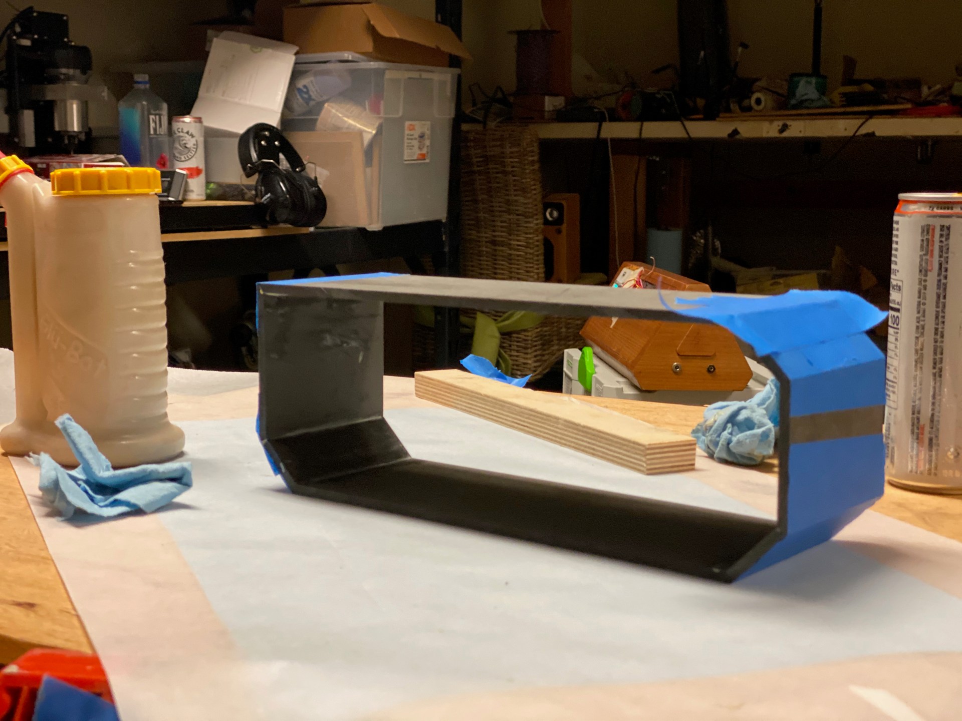


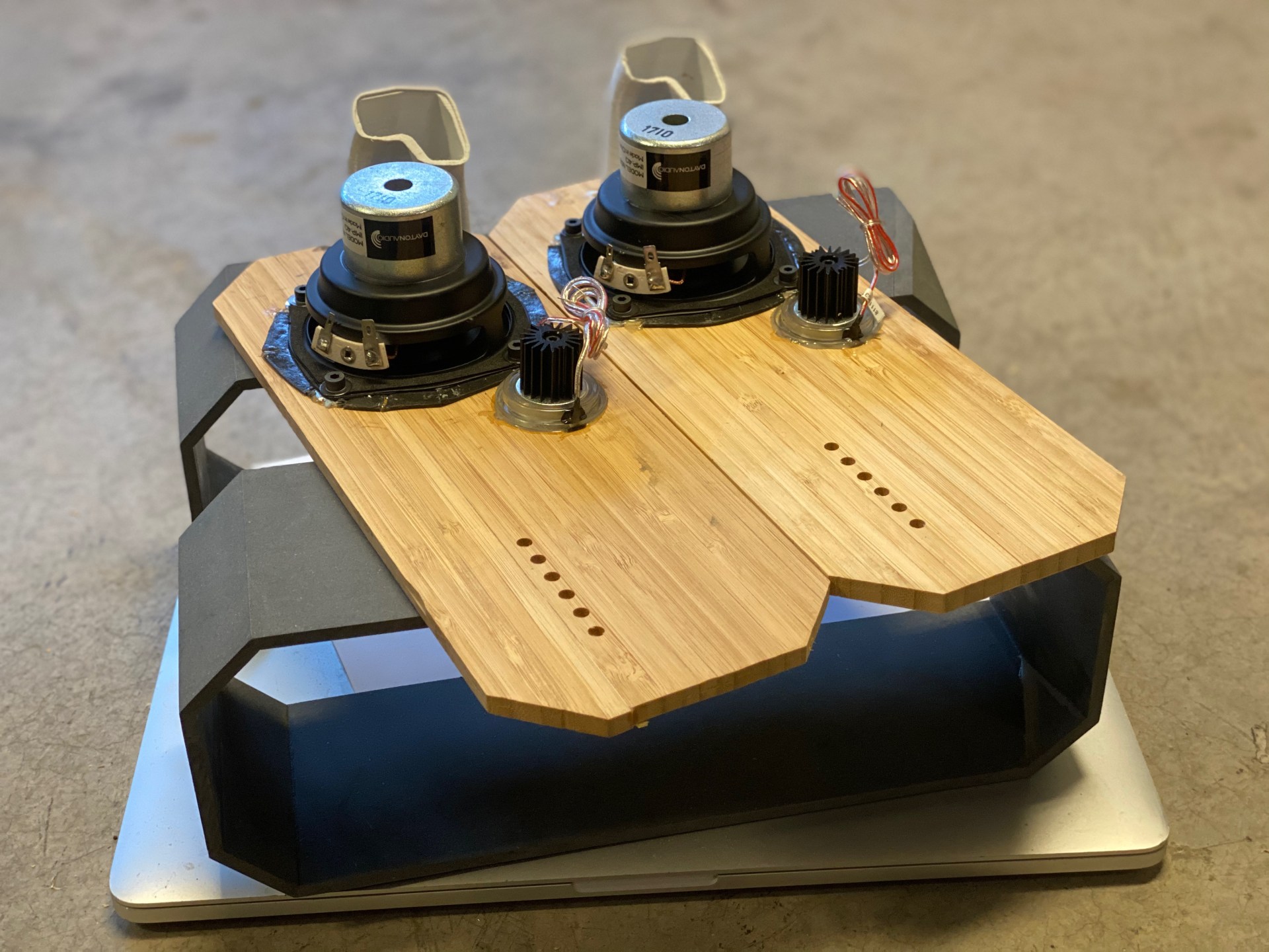


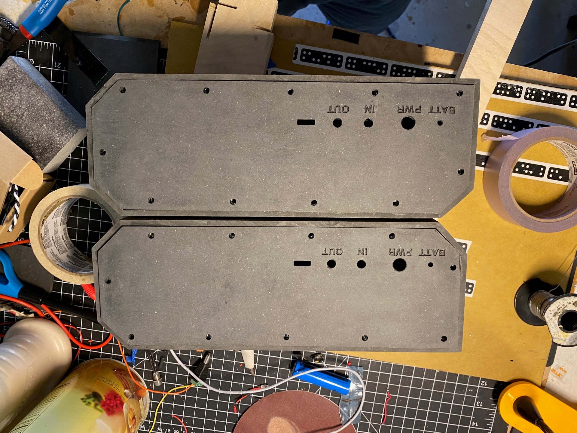
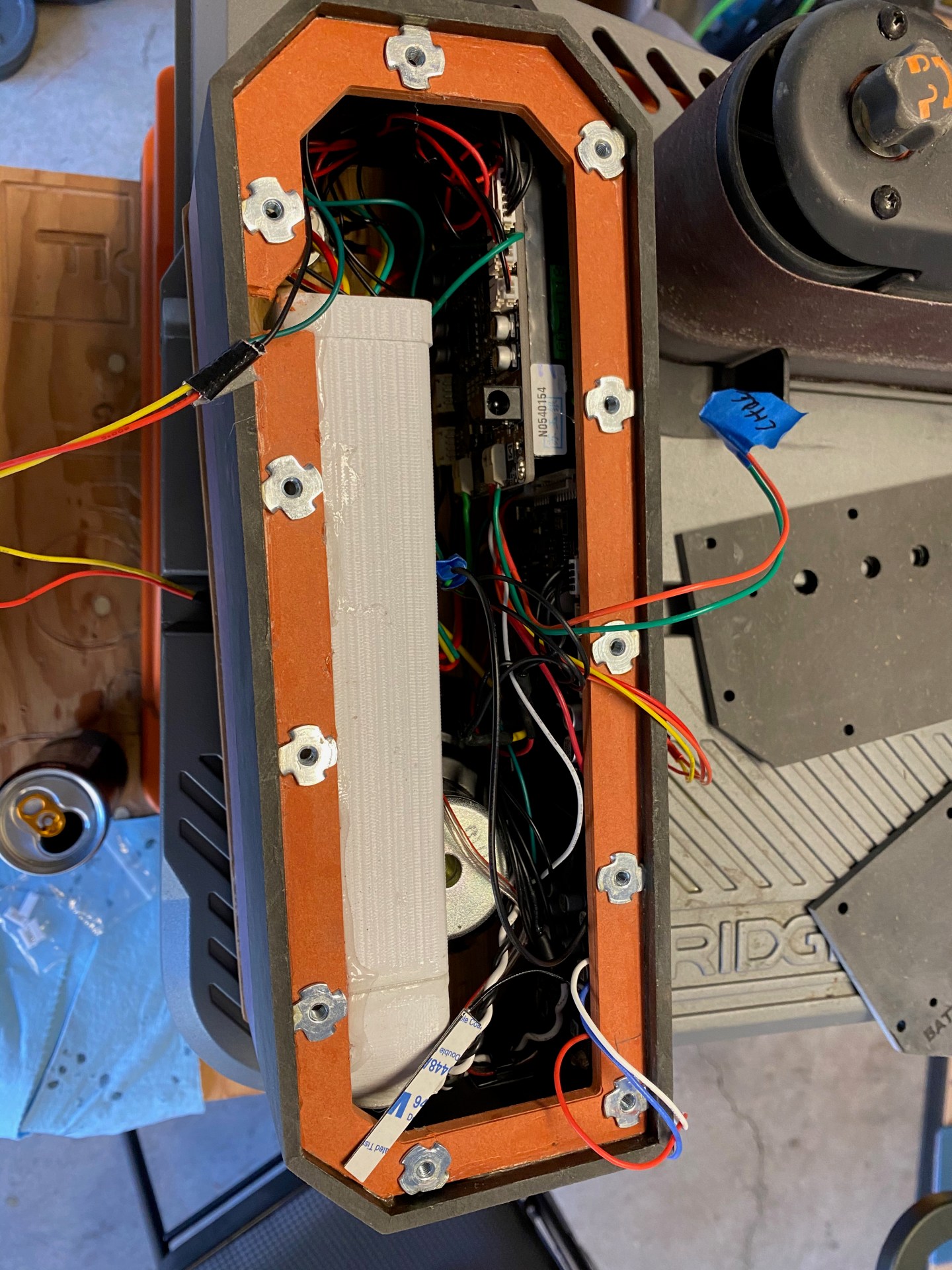


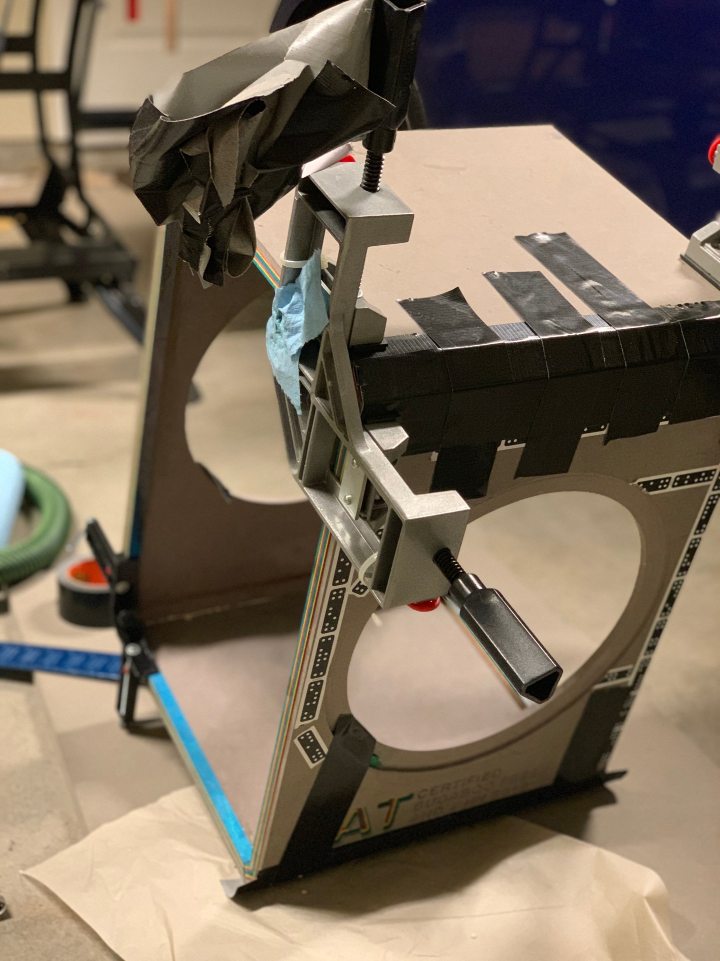
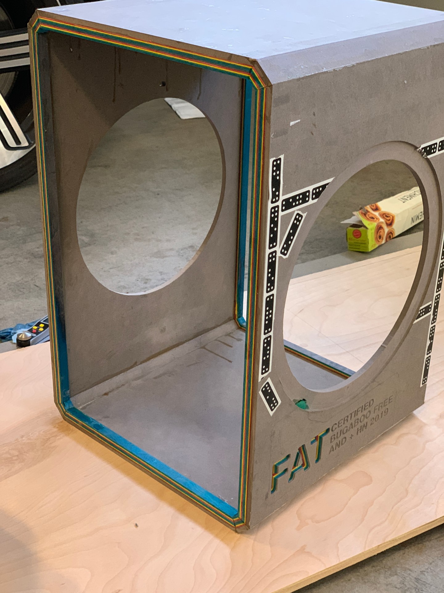


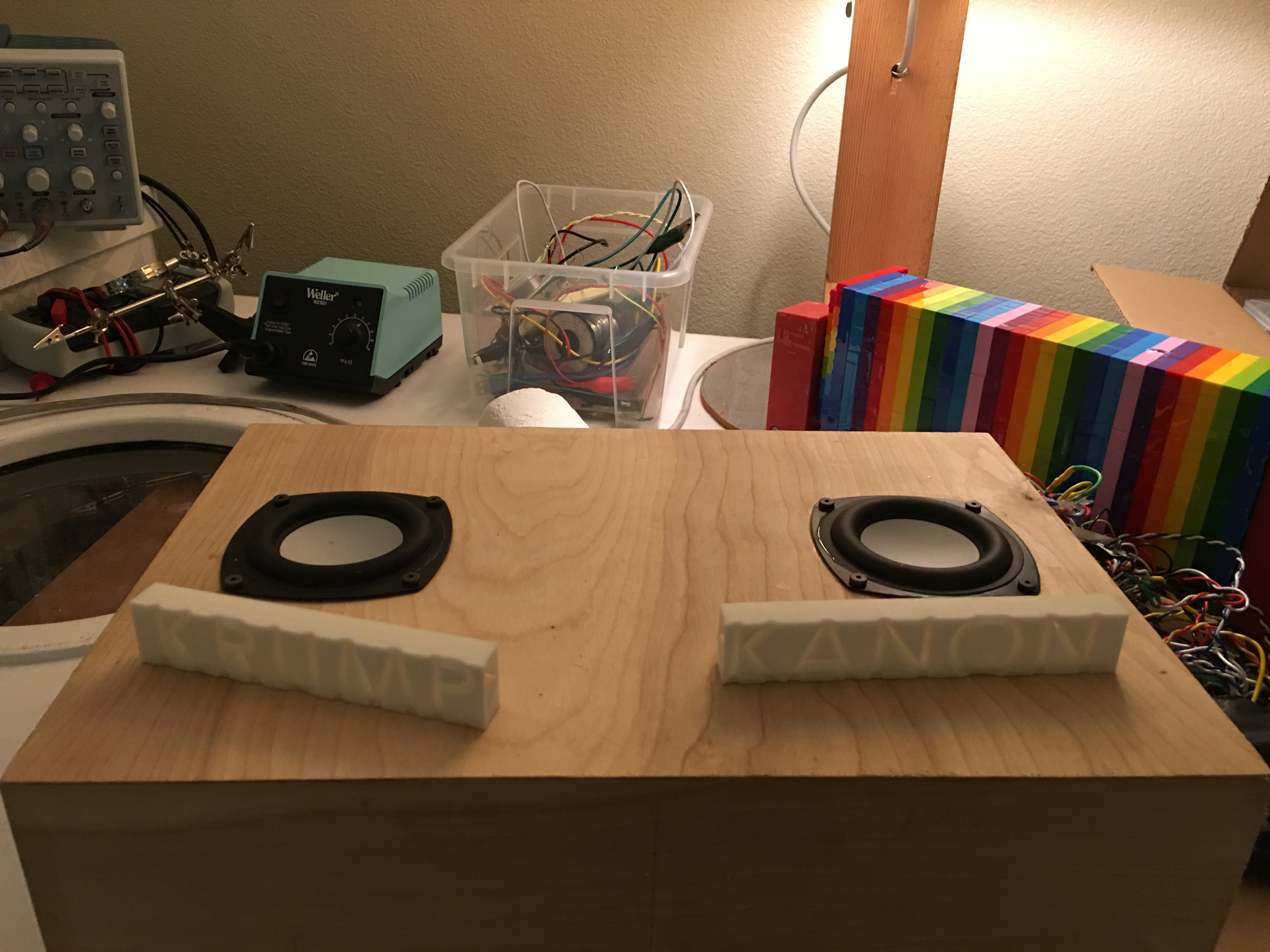
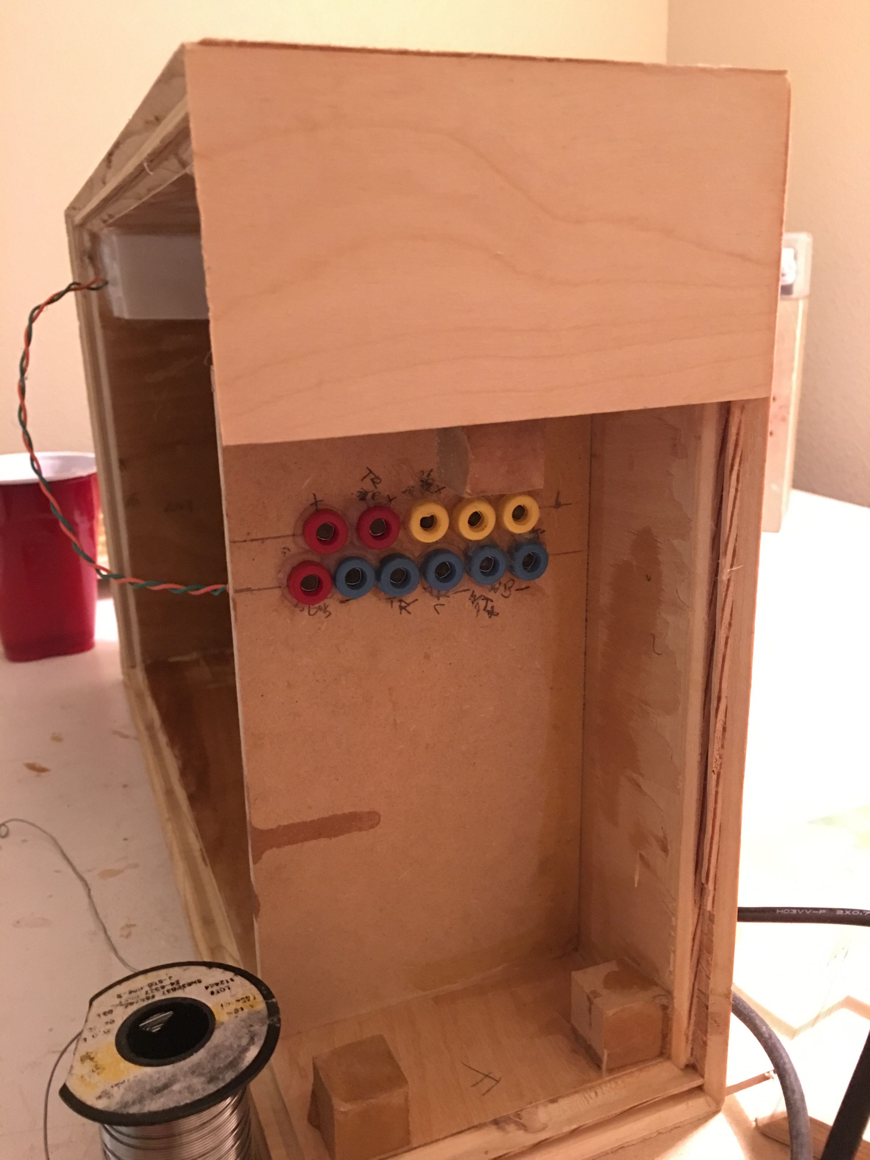
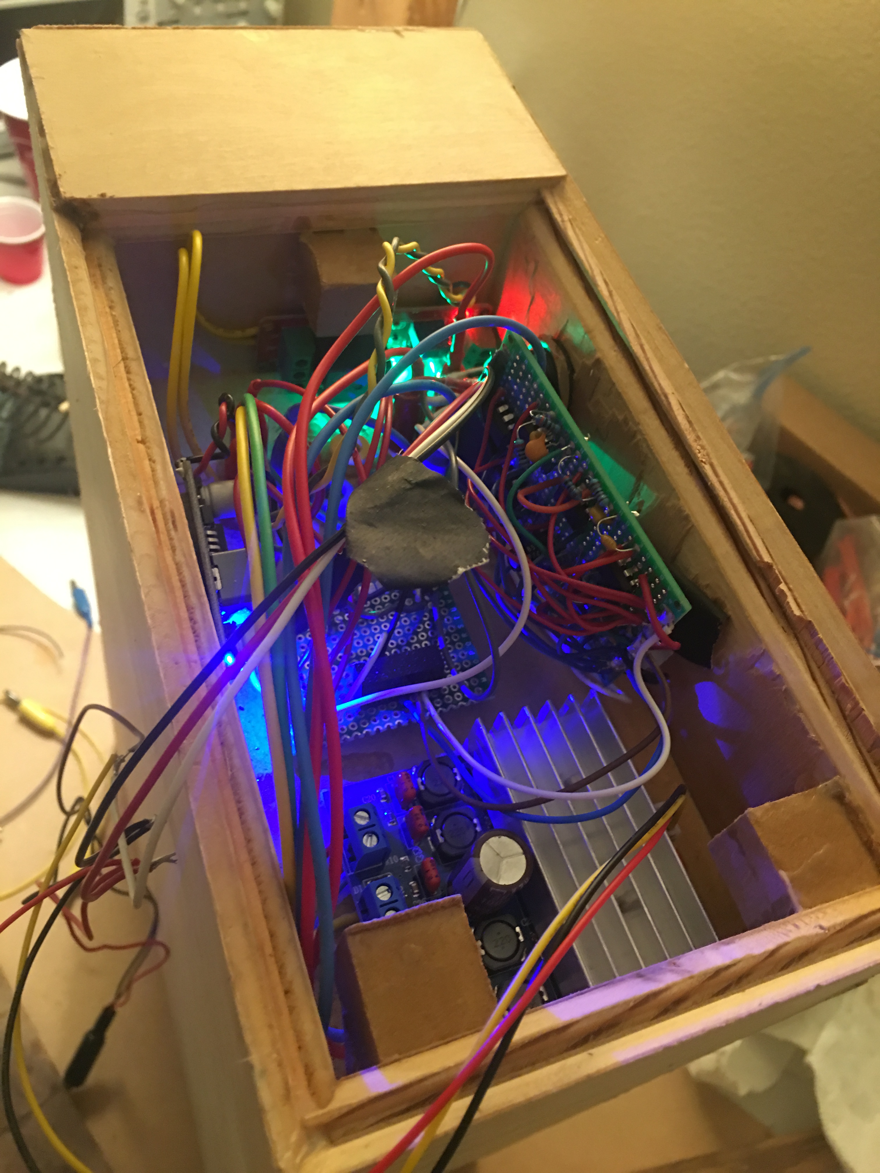
 The separated volume is for the electronics–lesson learned from previous projects is when trying to attain a good seal, either get better at electrical engineering, or compartmentalize your bad work.
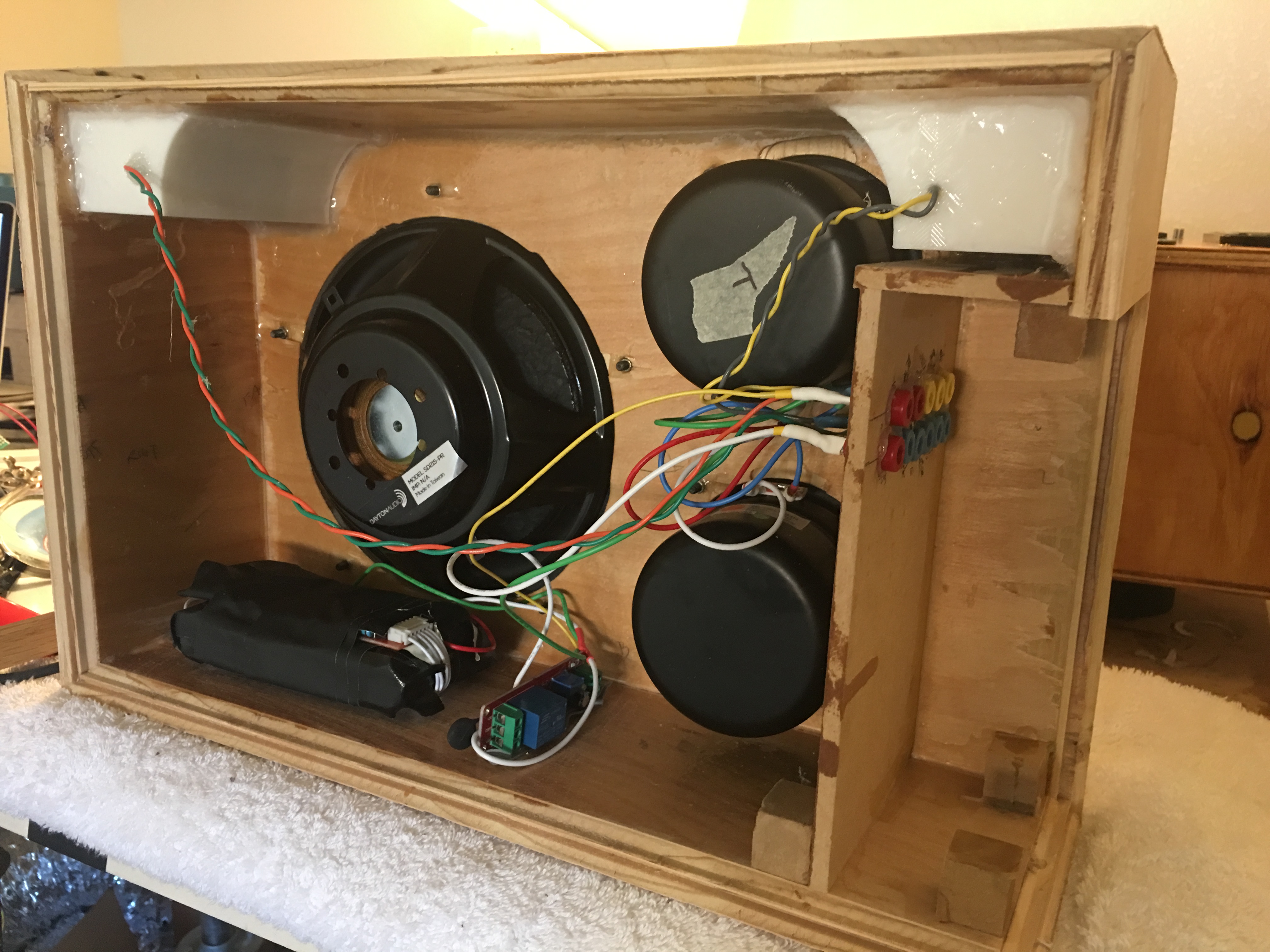


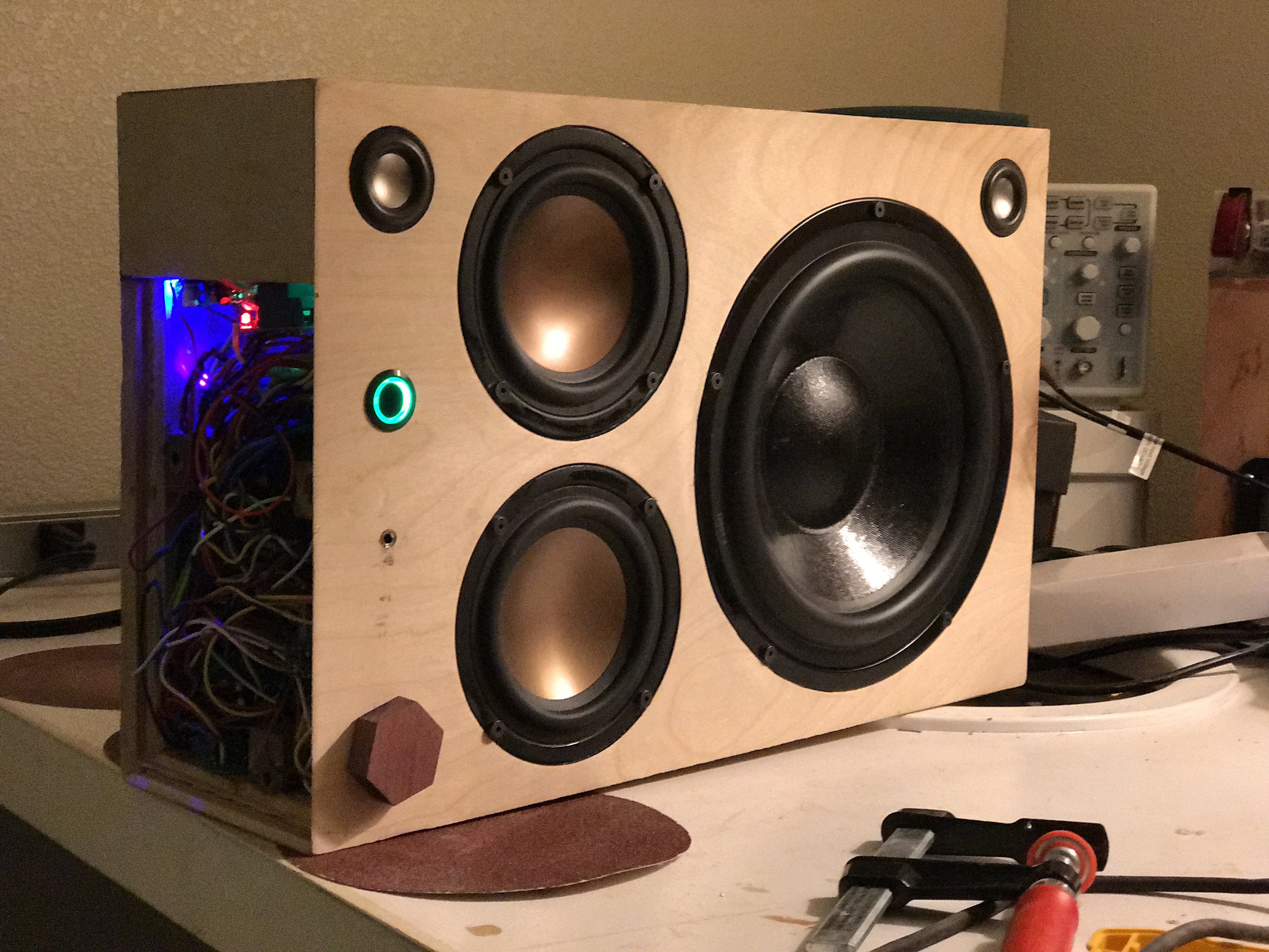


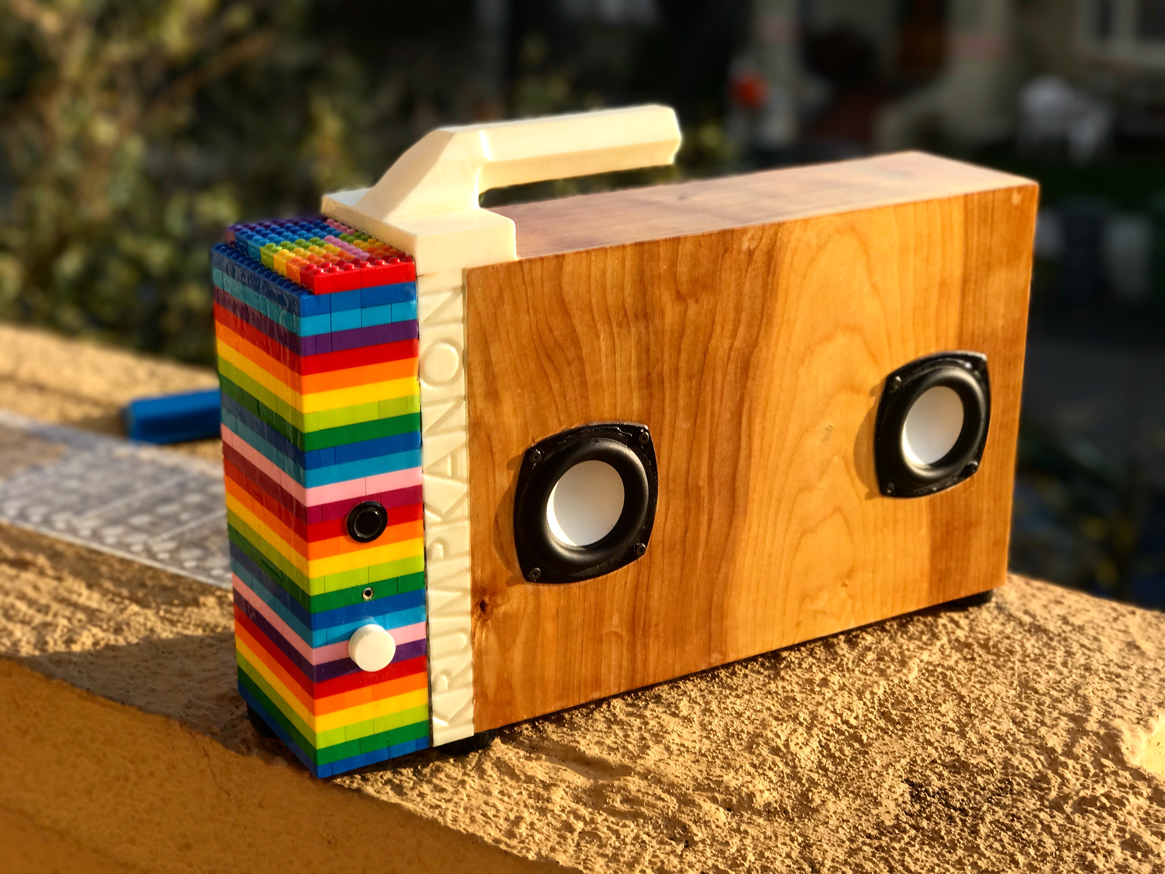
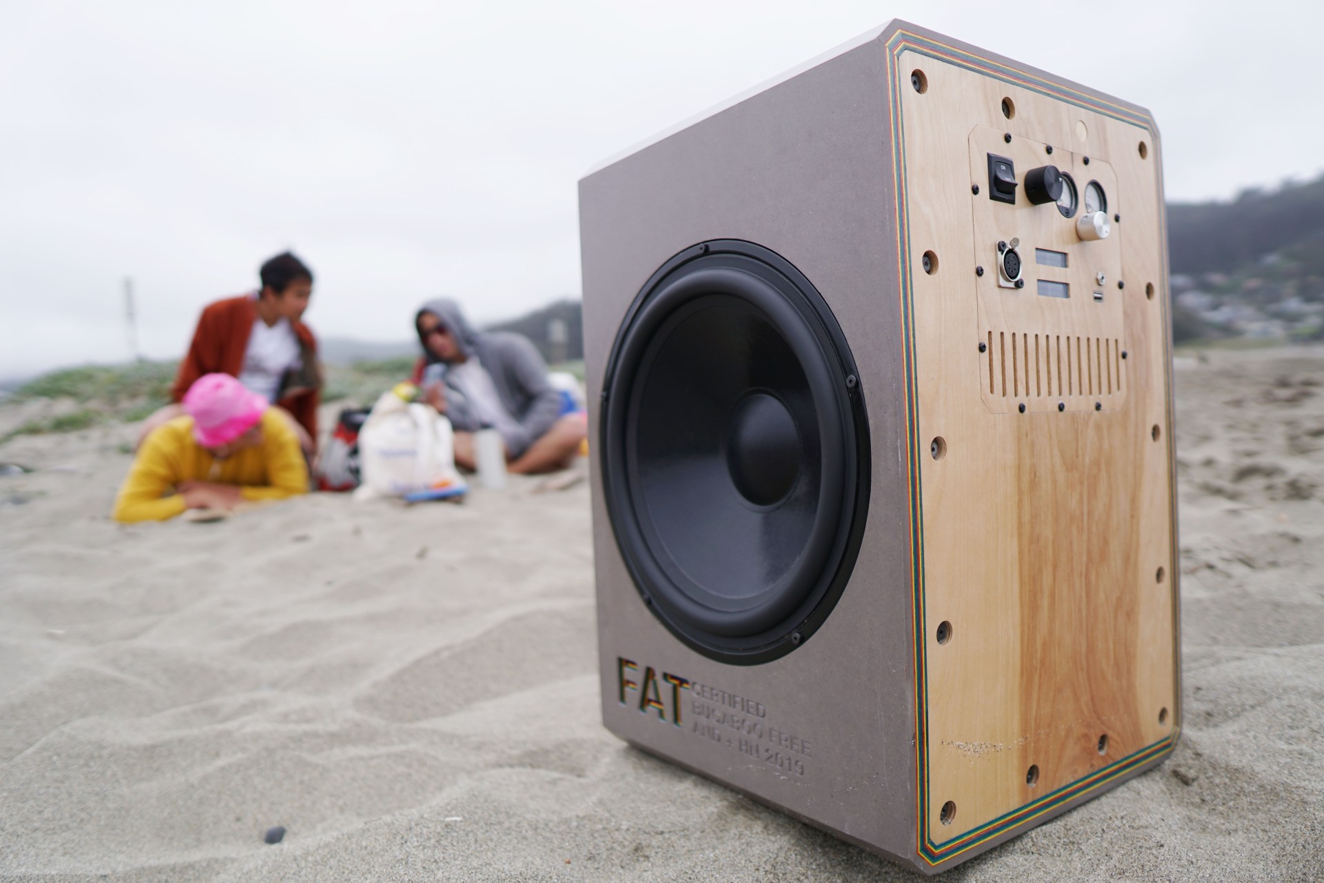
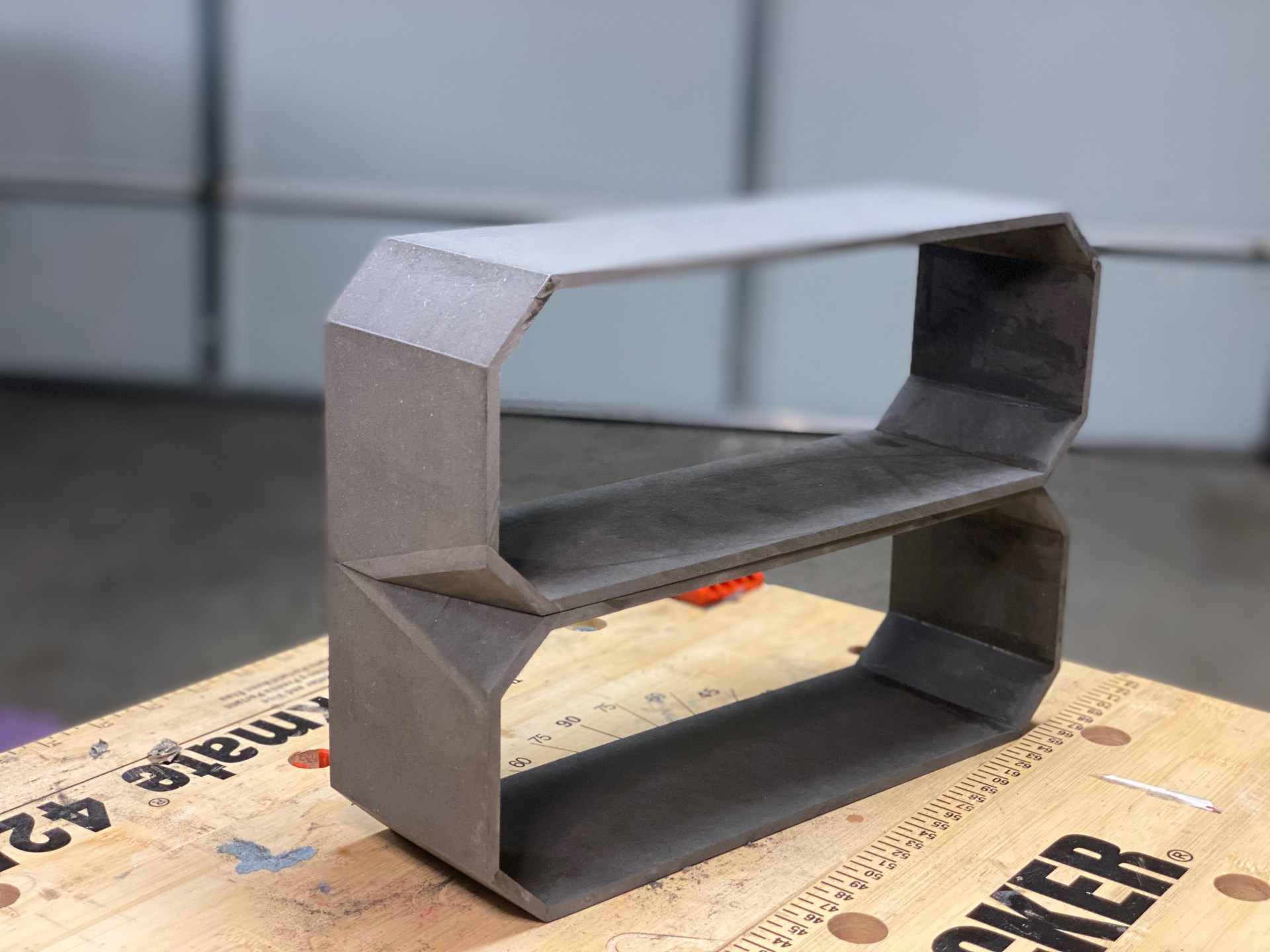
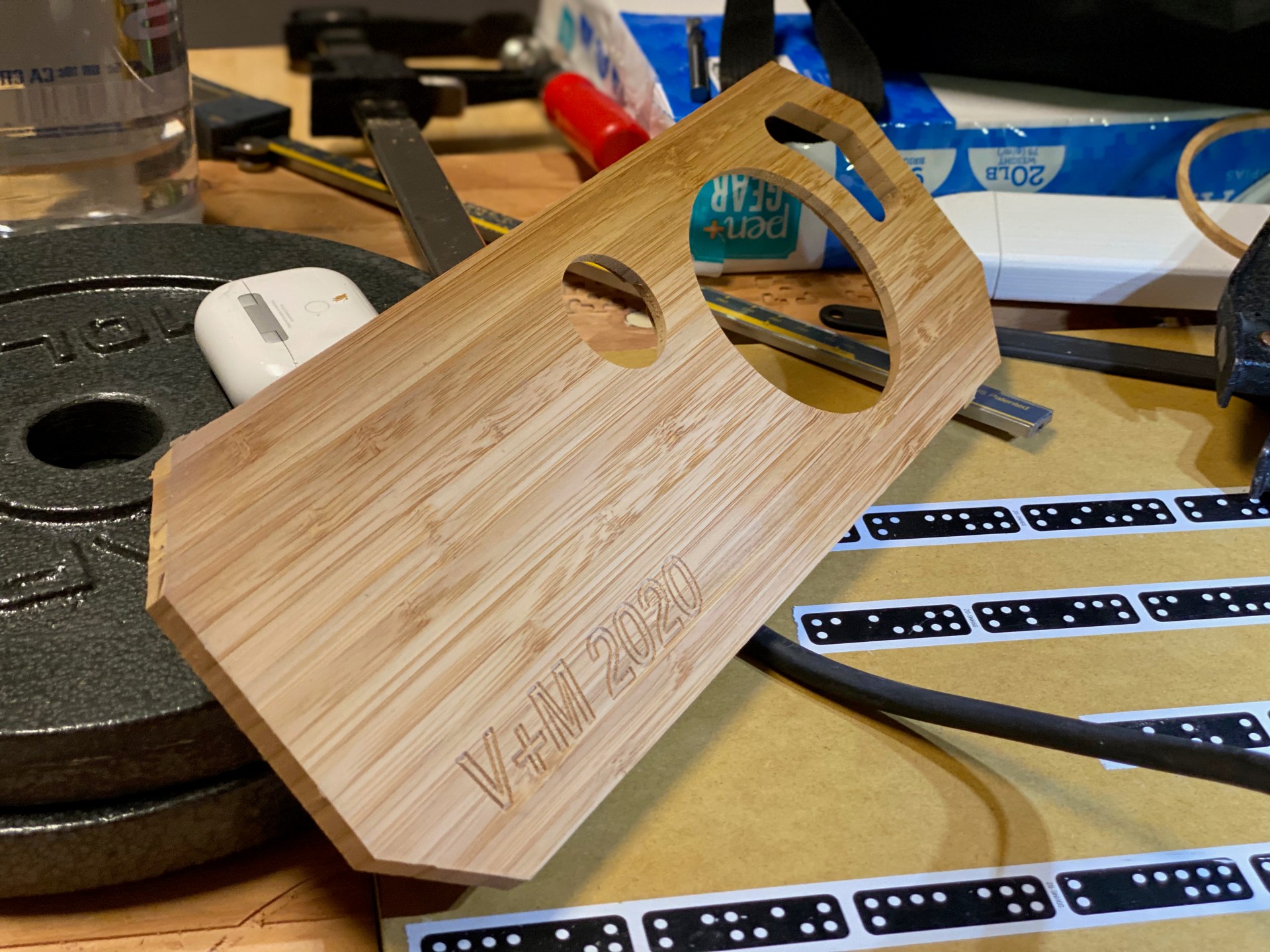
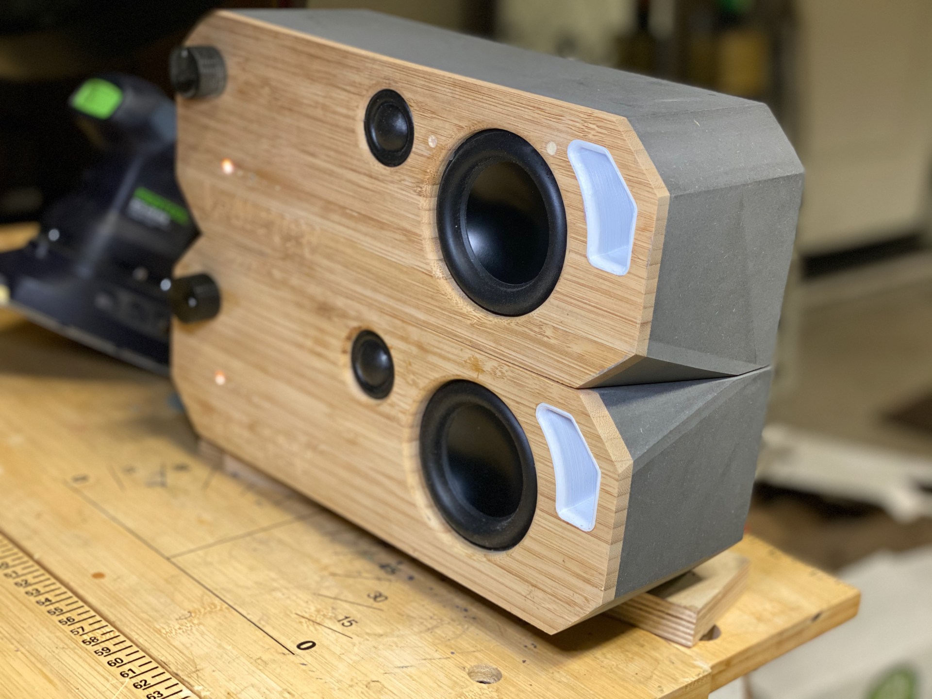
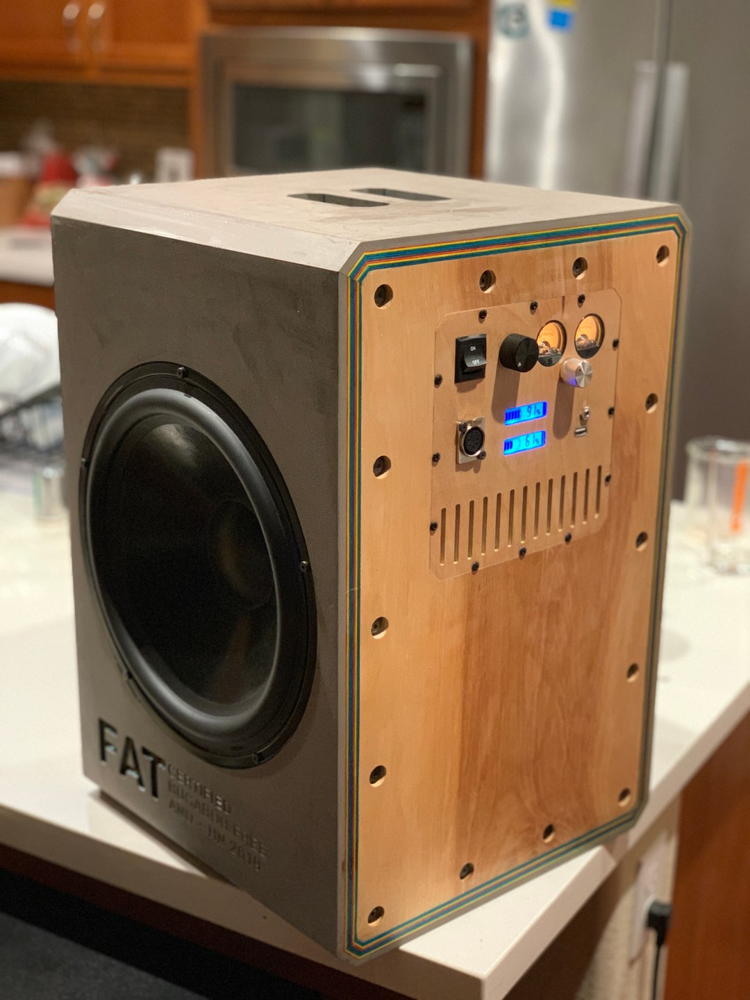
 Much like worried parents will fuss over a child before sending them off into the world, I fidgeted over the details of this lil guy, attempting to delay the inevitable departure, filled with pride and worry at the rigors he’ll face out in the real world. Unlike most worried parents, I eventually said “fuck it,” and dropped this fucker off at the local Fedex, to be shipped cross country in a large cardboard box.